Analytics
Setup a API
here is a list of available servers at absbox.org
from absbox import API,EnginePath

localAPI = API("https://absbox.org/api/latest")

# setting default language
localAPI = API("https://absbox.org/api/latest",lang='english')

# since version 0.26.7
# https://absbox.org/api/dev
localAPI = API(EnginePath.DEV,check=False)

# https://absbox.org/api/latest
localAPI = API(EnginePath.PROD,check=False)

# http://localhost:8081
localAPI = API(EnginePath.LOCAL,check=False)
Note
User can pull the docker image to run his/her own in-house environment
Note
the remote engine exposes RESTful Service , absbox send deal models and cashflow projection assumptions to that server.
The engine code was hosted at Hastructure
Asset Performance Assumption
Assumpitions are required to set when running stressed scenario as well as getting specific outputs other than cashflow.
There are two type of assumptions:
Assumptions for performance of asset
Assumptions for running a deal
pool assumption
See also
The assumption of asset start from point of time of Asset How assumption was applied on asset ?
Mortgage
Here is sample which used to set Pool level assumption on Mortgage asset class.
r = localAPI.run(deal
               ,poolAssump = ("Pool",("Mortgage",<default assump>,<prepay assump>,<recovery assump>,<extra assump>)
                                       ,<delinq assumption>
                                       ,<defaulted assumption>)
               ,runAssump = None
               ,read=True)
Note
Pool,means the assumption will be applied toallthe assets in the poolMortgage,means the it’s assumption applied toMortgageasset class
Performing
<Default Assumption>
default assumption for performing asset
{"CDR":0.01}means 1% in annualized of current balance will be defaulted at the end of each period{"CDR":[0.01,0.02,0.04]}means a vector of CDR will be applied since the asset snapshot date (determined byremain terms){"CDRPadding":[0.01,0.02,0.04]}same with above but the CDR 4% will be applied to rest of periods of the asset{"ByAmount":(2000,[0.25,0.25,0.50])}apply a custom default amount vector.{"DefaultAtEndByRate":(0.05,0.10)}, will apply 5% as CDR for all periods except last period. The last period will use default CDR 10% (which start from begining day).
New in version 0.42.2.
{"ByTerm":[ [vec1],[vec2]...], input list of vectors, asset will use vector with same origin term length
<Prepayment Assumption>
prepayment assumption for performing asset
{"CPR":0.01}means 1% in annualized of current balance will be prepay at the end of each period{"CPR":[0.01,0.02,0.04]}means a vector of CPR will be applied since the asset snapshot date (determined byremain terms){"CPRPadding":[0.01,0.02,0.04]}same with above but the CPR 4% will be applied to rest of periods of the asset
New in version 0.42.2.
{"PSA": 1.0}100% of PSA Speed.{"ByTerm":[ [vec1],[vec2]...], input list of vectors, asset will use vector with same origin term length
<Recovery Assumption>
recovery assumption for performing asset
{"Rate":0.7,"Lag":18}means 70% of current balance will be recovered at 18 periods after defaulted date{"Rate":0.45,"Timing":[0.3,0.3,0.4]}, recovery rate is 45% of current balance, and the recovery will be distributed to 3 periods after defaulted date with 30%,30% and 40% respectively
Non-Performing
<Delinquent Assumption>
assumption to project cashflow of asset in
delinquentstatusWarning
<delinq assumption> is not implemented yet ,it only serves as a place holder
reserve for future use : always use
None<Defaulted Assumption>
assumption to project cashflow of asset in
defaultedstatus("Defaulted":[0.5,4,[0.5,0.2,0.3]])
which says:
the recovery percentage is 50% of current balance
the recovery starts at 4 periods after defaulted date
the recovery distribution is 50%,20% and 30%
Summary
mortgage-assumption
Loan
r = localAPI.run(deal
               ,poolAssump = ("Pool",("Loan",<default assump>,<prepay assump>,<recovery assump>,<extra assump>)
                                       ,<delinq assumption>
                                       ,<defaulted assumption>)
               ,runAssump = None
               ,read=True)
Default
<default assump> :
{"CDR":<%>}, can be a vector or constant value<default assump> :
{"CDRPadding":<%>}, can be a vector or constant value, with last element till end of the asset
New in version 0.42.2.
{"ByTerm":[ [vec1],[vec2]...], input list of vectors, asset will use vector with same origin term length
Prepayment
<prepayment assump> :
{"CPR":<%>}, can be a vector or constant value<prepayment assump> :
{"CPRPadding":<%>}, can be a vector or constant value , with last element till end of the asset
New in version 0.42.2.
{"ByTerm":[ [vec1],[vec2]...], input list of vectors, asset will use vector with same origin term length
Summary
loan-assumption
Installment
r = localAPI.run(deal
               ,poolAssump = ("Pool",("Installment",<default assump>,<prepay assump>,<recovery assump>,<extra assump>)
                                       ,<delinq assumption>
                                       ,<defaulted assumption>)
               ,runAssump = None
               ,read=True)
Default
<default assump> :
{"CDR":<%>}
New in version 0.42.2.
{"ByTerm":[ [vec1],[vec2]...], input list of vectors, asset will use vector with same origin term length
Prepayment
<prepayment assump> :
{"CPR":<%>}
New in version 0.42.2.
{"ByTerm":[ [vec1],[vec2]...], input list of vectors, asset will use vector with same origin term length
Summary
installment-assumption
Receivable
user can set assumption on receivable asset class:
Default
assume default at last period ( 0 cash received )
a CDR way ,which is a percentage of current balance remains.
New in version 0.27.3.
Recovery
aussming a reocvery rate, with a distribution of recoverys by day offsets from defaulted day
# apply on asset level
r = localAPI.run(test01
            ,runAssump=[]
            ,poolAssump = ("ByIndex"
                              ,([0],(("Receivable", {"CDR":0.12}, None, None)
                                    ,None,None))
                              ,([1],(("Receivable", "DefaultAtEnd", None, None)
                                    ,None,None))
                              )
            ,read=True)

receivableAssump = ("Pool"
                    ,("Receivable", {"CDR":0.01}, None, None)
                    ,None
                    ,None)

receivableAssump = ("Pool",("Receivable" ,"DefaultAtEnd" ,{"Rate":0.5,"ByDays":[(10,0.5),(20,0.5)]} ,None)
                    ,None
                    ,None)


# apply on pool level
r = localAPI.run(test01
            ,runAssump=[]
            ,poolAssump = receivableAssump
            ,read=True)
Summary
receivable-assumption
Extra Stress
Supported Asset Class:
New in version 0.29.9.
user can specify a time series stress curve on prepay or default curve
syntax:
("StressByCurve",[<stress curve>,<assumption>])
<stress curve>: a list of [date,rate] pairs
<assumption>: the assumption to apply when the curve is active
# stress default curve
defAssump = {"CDR":0.017}
stressCurve = [["2020-10-01",1.0],["2023-03-01",4.0]]
stressDef = {"StressByCurve":[stressCurve,defAssump]}

p = localAPI.runPool(myPool,poolAssump=("Pool",("Mortgage",stressDef ,None,None,None)
                                              ,None
                                              ,None)
                    ,read=True)

# stress prepay curve
ppyAssump = {"CPR":0.017}
stressCurve = [["2020-10-01",1.0],["2023-03-01",4.0]]
stressPpy = {"StressByCurve":[stressCurve,ppyAssump]}

p = localAPI.runPool(myPool,poolAssump=("Pool",("Mortgage",None ,stressPpy,None,None)
                                              ,None
                                              ,None)
                    ,read=True)
Lease
Lease is an asset type that model contractual cash inflow from leasing out equipments or houses. It is differente from other asset type Loan or Mortgage in the performance assumption.
No-Prepayment There is little economic motivation to prepay the rental in advance
Revovling by default The Lease shall base on some physical entity, like the Room/Hotel or CellPhone , which can be used to generate a series of Lease contracts
r = localAPI.run(deal
               ,poolAssump = ("Pool",("Lease", <default assumption>,<turnover gap>, <rental assump>, <end type>)
                                       ,<delinq assumption>
                                       ,<defaulted assumption>
                                       )
               ,runAssump = None
               ,read=True)
Notes:
<default assumption>-> optional, assumption on gap days between new lease and old lease
<turnover gap>-> assumption on gap days between new lease and old lease
<rental assump>-> describe the rental increase/decrease over time
<end type>
("byDate", "2026-09-20")-> the date when lease projection ends
("byExtTimes",1)-> how many times lease will roll over
Lease Rental
Rental is being used to factor in the future rental upside and downside risk.
In this example: it assume the market rental rate is dropping by 30% each year. When a new lease contract was created, the new rental rate depends on the two attributes from last lease.
('byAnnualRate', -0.3)
rental rate from last lease
originate date from last lease
syntax:
('byAnnualRate', <annual rate>): the rental will increase/decrease by a fixed rate in annual
('byRateCurve', <curve>): the rental will increase/decrease by a curve, which is a list of [date,rate] pairs
('byRateVec', -0.1,-0.3,-0.2): the rental will increase/decrease by a vector of rates, which is applied to each new projected lease.
Lease Default
User can pass it as None or default assumptions as below:
('byContinuation', <default rate in annual>)('byTermination', <default rate in annual>)
Note
byContinuate vs byTermination There are two type of asset being leased out, categorized by how default behaviors affecting cashflow. Like, office lending. The default behavior of first lease won’t affect second lease. But for phone leasing, once the default happends, the phone will be lost and can’t be lease any more. In the phone case, the default of first lease will affect cashflow of leases afterwards.
byContinuation : for the phone lease case.
byTermination : for the office/hotel room lease case.
Lease Gap
Gap was to model the blank period between last lease and new lease. In such period, there isn’t any cash flow in. It varies because to model different type of asset. Like, commerial office , on average , has longer gap days than a smart phone.
('days', x): the number of days between old lease and new lease('byCurve', c): the number of days between old lease and new lease depends on a curve
Lease End
Describle the end type of lease projection,either by a Date or a Extend Time
("byDate", "2026-09-20"): the date when lease projection ends("byExtTimes", 1): how many times lease will roll over for 1 time
New in version 0.46.1.
("earlierOf", "2026-09-20", 3): the lease projection ends at the earlier of the date or extend time("laterOf", "2026-09-20", 3): the lease projection ends at the later of the date or extend time
Summary
lease-assumption
Fixed Asset
- syntax
(“Fixed”,<Utilization Rate Curve>,<Cash value per Unit>)
myAssump = ("Pool"
            ,("Fixed",[["2022-01-01",0.1]]
                     ,[["2022-01-01",400] ,["2024-09-01",300]])
            ,None
            ,None)

p = localAPI.runAsset("2021-04-01"
                      ,assets
                      ,poolAssump=myAssump
                      ,read=True)
Summary
fixedAsset-assumption
How to setup assumption for assets
Pool assumption can be applied via multiple ways:
By Pool Level
By Asset Index
By Obligor
asset-assumption
By Pool Level
The assump will be applied to ALL assets in the pool
# For Loan type asset
("Pool",("Loan",<default assump>,<prepay assump>,<recovery assump>,<extra assump>)
                                ,<delinq assumption>
                                ,<defaulted assumption>)

("Pool",("Mortgage",<default assump>,<prepay assump>,<recovery assump>,<extra assump>)
                                ,<delinq assumption>
                                ,<defaulted assumption>)

("Pool",("Installment",<default assump>,<prepay assump>,<recovery assump>,<extra assump>)
                                ,<delinq assumption>
                                ,<defaulted assumption>)

# others
Asset Level By Index
The assumption will be applied to assets by their index position in the pool
#syntax
("ByIndex"
  ,([<asset id>..],(<performing assump>,<delinq assump>,<defaulted assump>))
  ,([<asset id>..],(<performing assump>,<delinq assump>,<defaulted assump>))
  ,....
  )
i.e
myAsset1 = ["Mortgage"
            ,{"originBalance": 12000.0
             ,"originRate": ["fix",0.045]
             ,"originTerm": 120
             ,"freq": "monthly"
             ,"type": "level"
             ,"originDate": "2021-02-01"}
            ,{"currentBalance": 10000.0
             ,"currentRate": 0.075
             ,"remainTerm": 80
             ,"status": "current"}]
myAsset2 = ["Mortgage"
            ,{"originBalance": 12000.0
             ,"originRate": ["fix",0.045]
             ,"originTerm": 120
             ,"freq": "monthly"
             ,"type": "level"
             ,"originDate": "2021-02-01"}
            ,{"currentBalance": 10000.0
             ,"currentRate": 0.075
             ,"remainTerm": 80
             ,"status": "current"}]

myPool = {'assets':[myAsset1,myAsset2],
          'cutoffDate':"2022-03-01"}

Asset01Assump = (("Mortgage"
                 ,{"CDR":0.01} ,{"CPR":0.1}, None, None)
                 ,None
                 ,None)
Asset02Assump = (("Mortgage"
                 ,{"CDR":0.2} ,None, None, None)
                 ,None
                 ,None)

AssetLevelAssumption = ("ByIndex"
                        ,([0],Asset01Assump)
                        ,([1],Asset02Assump))

r = localAPI.runPool(myPool
                   ,poolAssump=AssetLevelAssumption
                   ,read=True)

# asset cashflow
r[0]
By Obligor
User can apply assumption on assets with specific obligor tags/id with optional default clause.
New in version 0.29.1.
User supply a list of rules to match assets, each rule will match a set of assets and apply the same assumption.
Sequence is important, earlier rule has higher priority, the assets not match any of above rules will be test agaist the rules next.
By ID: hit when obligor id is in the list
By Tag: <Match Rule>
TagEqhit when asset tags equals to tags in the assumptionTagSubsethit when asset tags is a subset of the listTagSupersethit when asset tags is a superset of the listTagAnyhit when asset tags has any intersetion with tags in assumption("not", "<Tag>")hit when negate the above rules
By Default : default asset performance if assets are not hit by any of above rules before
#syntax
("ByObligor",("ByTag",<tags>,<match rule>,<assumption>)
            ,("ById",<ids>,<assumption>)
            ,("ByDefault",<assumption>))
See also
By Obligor Fields
New in version 0.29.2.
Syntax is similar to By Obligor, but the match rule is based on asset fields.
- Field Match Rule:
(“not”, <Field Match Rule>) : negate the rule
(<fieldName>, “in”, <option list>): hit when asset field value in the list
(<fieldName>, “cmp”, <cmp>, <value>): only for numeric field value, hit when asset field value compare with value by cmp operator
(<fieldName>, “range”, <rangeType>, <lowValue>, <highValue>): only for numeric field value, hit when asset field value in the range
("ByObligor",("ByTag",<tags>,<match rule>,<assumption>)
            ,("ById",<ids>,<assumption>)
            ,("ByField",[<field match rule>],<assumption>)
            ,("ByDefault",<assumption>))
By Pool Name
This assumption map with key of assumption to the name of pool. It will apply Pool Level assumption to pools with same name
#syntax
("ByName",<assumption map>)
- Assumption map
Key -> Pool Name/Id Value -> (<performing assumption> ,<delinq assumption> ,<defaulted assumption>)
By Pool Id
This assumption map with key of assumption to the name of pool. It will apply Any Level assumption to pools with same name
#syntax
("ByPoolId",<assumption map>)
- Assumption map
Key -> Pool Name/Id Value -> <Any Pool Assumption>
By Deal Name
This only apply to resercuritization deal, which the key of assumption is the name of underlying deal.
#syntax
("ByDealName",<assumption>)
Deal Assumption
Deal Assumption is just list of tuples passed to runAssump argument.
r = localAPI.run(deal
                 ,poolAssump = None
                 ,runAssump = [("stop","2021-01-01")
                              ,("call",("CleanUp",("poolBalance",200)))
                              ,.....]
                 ,read=True)
Stop Run
A debugging assumption to stop the deal projection. Either stop by a specific date or by a Condition.
cashflow projection will stop at the date specified.
("stop","2021-01-01")
New in version 0.46.5.
After 0.46.5, the stop run can be specified by a Condition which will be evaluated on each distribution date described by DatePattern. Any condition met will stop the projection.
("stop", <DatePattern>, *<Condition>)
# on each month end, the engine will evaluate two conditions
# , stop projection when ALL of them are met

("stop", "MonthEnd"
       , [">=","2022-01-01"], [("bondBalance","A1"),"<=",200])
Project Expense
a time series of expense will be used in cashflow projection.
# fee in the deal model
,(("trusteeFee",{"type":{"fixFee":30}})

    ,("tsFee",{"type":{"customFee":[["2024-01-01",100]
                                  ,["2024-03-15",50]]}})
    ,("tsFee1",{"type":{"customFee":[["2024-05-01",100]
                                    ,["2024-07-15",50]]}})
   )

# assumption to override
r = localAPI.run(test01
             ,runAssump=[("estimateExpense",("tsFee"
                                             ,[["2021-09-01",10]
                                              ,["2021-11-01",20]])
                                            ,("tsFee1"
                                             ,[["2021-12-01",10]
                                              ,["2022-01-01",20]])
                         )]
             ,read=True)
Call When
Assumptions to call the deal and run CleanUp waterfall. If no CleanUp waterfall is setup ,then no action perform.
either of Condition was met, then the deal was called.
the call test was run on distribution day, which is described by payFreq on Deal Dates
("call",{"poolBalance":200},{"bondBalance":100})

("call",{"poolBalance":200} # clean up when pool balance below 200
       ,{"bondBalance":100} # clean  up when bond balance below 100
       ,{"poolFactor":0.03} # clean up when pool factor below 0.03
       ,{"bondFactor":0.03} # clean up when bond factor below 0.03
       ,{"afterDate":"2023-06-01"} # clean up after date 2023-6-1
       ,{"or":[{"afterDate":"2023-06-01"} # clean up any of them met
               ,{"poolFactor":0.03}]}
       ,{"and":[{"afterDate":"2023-06-01"} # clean up all of them met
               ,{"poolFactor":0.03}]}
       ,{"and":[{"afterDate":"2023-06-01"} # nested !!
                ,{"or":
                   [{"poolFactor":0.03}
                   ,{"bondBalance":100}]}]})
New in version 0.23.
Or more powerfull condition with Condition ! Yeah, we are reuse as many components as possible to flat the learning curve. 😎
("call", ("if", <Condition>))
("call", ("condition", <Condition>))
Let’s build some fancy call condition with a Formula value less than a threshold.
("call", ("if",
          [("substract",("poolWaRate",),("bondWaRate","A1","A2","B")), "<", 0.01]
          )
)
New in version 0.30.7.
New callWhen was introduced, which has two options:
onDates, the Condition will be tested on each date described by DatePatternif, the Condition will be tested on waterfall payment date.
Any Condition triggered will fire the cleanUp waterfall actions and ends the deal run.
("callWhen", ("onDates", <DatePattern>, <Condition 1>, <Condition 2>...))
("callWhen", ("if", <Condition 1>, <Condition 2>...))


("callWhen", ("if", <Condition 1>, <Condition 2>...)
           , ("onDates", <DatePattern>, <Condition 1>, <Condition 2>...)
)

("callWhen", ("if", <Condition 1>, <Condition 2>...)
           , ("onDates", <DatePattern 1>, <Condition 1>, <Condition 2>...)
           , ("onDates", <DatePattern 2>, <Condition 3>, <Condition 4>...)
)
Note
Example Test Calls
Note
Why Call is an assumption ?
In deal arrangement, call is an option which doesn’t have to be triggered. It may grant issuer call option if net loss rate above 5%, but issuer may call the deal when loss rate is 7%. That’s why when projecting cashflow, it leave option to user assumption.
Revolving Assumption
User can set assumption on revolving pool with two compoenents: assets and performance assumption.
- pool of revolving assets
["constant",asset1,asset2....]- there are three types of revolving pools:
constant: assets in the pool will not change after buystatic: assets size will be shrink after buycurve: assets available for bought will be determined by a time based curve
- assumption for revolving pool
<same as pool performance>
Warning
the assumption for revolving pool only supports “Pool Level”
("revolving"
 ,["constant",revol_asset]
 ,("Pool",("Mortgage",{"CDR":0.07},None,None,None)
           ,None
           ,None))
User has the option to set multiple revovling pool in assumption which represents different characteristics of assets to buy.
("revolving"
    ,{"rA":(["constant",revol_asset1]
            ,("Pool",("Mortgage",{"CDR":0.07},None,None,None)
                      ,None
                      ,None)),
      "rB":(["constant",revol_asset2]
            ,("Pool",("Mortgage",{"CDR":0.03},None,None,None)
                      ,None
                      ,None)),
      "rC":(["constant",revol_asset3]
            ,("Pool",("Mortgage",{"CDR":0.01},None,None,None)
                      ,None
                      ,None)),
    }
)
Refinance Bonds
New in version 0.29.3.
The bond’s interest rate compontent can be changed at a future date. Floater rate can be changed to fix rate, or coupon rate can be changed to higher or lower rate.
- syntax:
("refinance",<refinance 1>,<refinance 2>...)
- <refinance>
("byRate",<Date>,<AccountName>,<BondName>,<InterestInfo>)<Date> : when the bond’s interest rate changes
<AccountName> : the account used to settle interest accrued at changing date
<BondName>: which bond’s interest to be changed
<InterestInfo>: the new interest info of the bond, same in the bond component
See also
Interest Rate
set interest rate assumptions for cashflow projection. It can be either a flat rate or a rate curve.
- syntax:
("interest",(<index>, rate))("interest",(<index>, rateCurve))
New in version 0.30.8.
("rate",(<index>, rate))("rate",(<index>, rateCurve))
from absbox import Generic
## interest on asset
r = localAPI.run(test01
               ,runAssump=[("interest"
                           ,("LPR5Y",0.04)
                           ,("SOFR3M",[["2021-01-01",0.025]
                                       ,["2022-08-01",0.029]]))]
               ,read=True)
Inspection
Transparency matters ! For the users who are not satisfied with cashflow numbers but also having curiosity of the intermediary numbers, like bond balance, pool factor .
Users are able to query values from any point of time ,using
- syntax:
(<DatePattern>,<Formula>)
New in version 0.29.14.
(<DatePattern>,[<Formula>,<Formula>...])
any point of time -> annoate by DatePattern
values -> annoate by Formula
("inspect",("MonthEnd",("poolBalance",))
          ,("QuarterFirst",("bondBalance",))
          ,("QuarterEnd",[ ("bondBalance",), ("bondFactor",)])
          ,....)

r = localAPI.run(test01
             ,poolAssump = ("Pool",("Mortgage",{"CDR":0.01},None,None,None)
                                     ,None
                                     ,None)
             ,runAssump = [("inspect",["MonthEnd",("poolFactor",)]
                                     ,["MonthEnd",("trigger","AfterCollect","DefaultTrigger")]
                                     ,['MonthEnd',("cumPoolDefaultedRate",)]
                                     ,['MonthEnd',("status","Amortizing")]
                                     ,['MonthEnd',("rateTest",("cumPoolDefaultedRate",),">=",0.00107)]
                                     ,['MonthEnd',("anyTest", False
                                                   ,("rateTest",("cumPoolDefaultedRate",),">=",0.00107)
                                                   ,("trigger","AfterCollect","DefaultTrigger")
                                                  )]
                           )]
             ,read=True)
To view these data as map, with formula as key and a dataframe with time series as value.
# A map
r['result']['inspect']
# a dataframe
r['result']['inspect']['<CurrentBondBalance>']
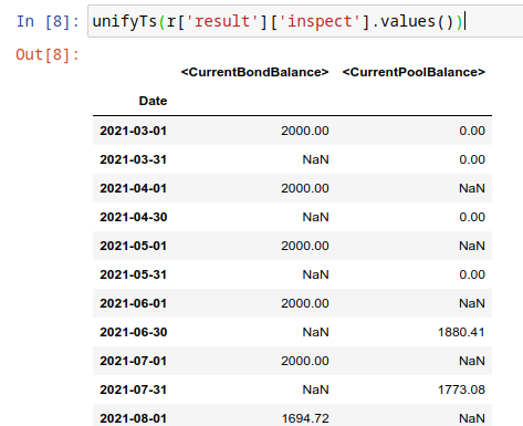
# join all vars into a single dataframe
But, the values are a dataframe with single column, how to view all the variables in a single dataframe ? Here is the answer :
from absbox import unifyTs,readInspect

unifyTs(r['result']['inspect'].values())

# .. versionadded:: 0.29.15, it will show vars from 'inspect' and 'inspectWaterfall'
readInspect(r['result'])
Note
readInspectis the prefer way, it shows the data in a easy way which include both inspect and inspectWaterfall data.Notebook Exmaple Inspect Example
Financial Reports
User just need to specify the dates of financial statement by DatePattern
Note
There is a major refactor on financial reports on version 0.31.4
- BalanceSheet
The engine will query all the deal component (Accounts,Asset Pools,Bonds,Fees,misc). Then engine will calculate possbile accrue value ( accrue interest for bonds or accounts ,accure expenses) Misc components includes the Interest Rate Swap and Liquidity Provider
- CashflowReport
The cashflow report will aggregate all transactions in the accounts during time period. Engine will group these transactions into Inflow and Outflow.
("report",{"dates":"MonthEnd"})
to view results
r['result']['report']['balanceSheet']

r['result']['report']['cash']
Pricing & IRR
User can provide a pricing curve and a pricing data to argument pricing,which all future bond cashflows will be discounted at that date with the curve provided.
("pricing"
  ,{"date":"2021-08-22"
    ,"curve":[["2021-01-01",0.025]
             ,["2024-08-01",0.025]]})
Caculate Z-spread
User need to provide a {<bond name>:(<price date>,<price>)}
The engine will calculate the how much spread need to added into curve, then the PV of
bond cashflow equals to <price>
("pricing"
  ,{"bonds":{"A1":("2021-07-26",100)}
   ,"curve":[["2021-01-01",0.025]
            ,["2024-08-01",0.025]]})
Calculate IRR of bonds
New in version 0.42.4.
User shall input a dict with solo key IRR and value is a dict with bond name and IRR calculate assumption
("pricing"
    ,{"IRR":
        {"B":<IRR calculate assumption>
      }
    }
  )
- IRR calculate assumption
It has three types
- Holding a bond to maturity
("holding",[<history of cashflow of investment>], <position size>){"B":("holding",[("2021-04-01",-500)],500)
- Holding a bond and sell it at a future date
("holding",[<history of cashflow of investment>],<position size>,<sell date>,<sell price>)}("holding",[("2021-04-01",-500)],500,"2021-08-19",("byFactor",1.0))}
- Buy a bond at a future date and hold it to maturity
("buy",<buy date>,<buy price>,<cash to buy>)("buy","2021-08-01",("byFactor",0.99),("byCash",200))
See also
Example IRR Example
Mannual Fire Trigger
New in version 0.23.
It’s not that often but someone may need to mannually fire a trigger and run the effects of a trigger.
- syntax
("fireTrigger", [(<Date Of Fire>,<Loc of Trigger>,<Trigger Name>)])
("fireTrigger",[("2021-10-01","AfterCollect","poolDef")
See also
Example Mannual fire a trigger
Make Whole Call
New in version 0.26.0.
User can specify a Make Whole Call date , and a fixed spread following, and a WAL/Spread mapping.
The engine will stop projection at the make whole call date.
Then project with no-stress on the pool and simulate the future bond cashflow.
calculate bond’s WAL and find each bond’s spread based on the input table
then for each bond’s spread will be add with fixed spread.
using the total spread ( spread from lookup table and fixed spread) to discount future bond cashflow to get the PV
the PV will be paid off the bond ,if PV > oustanding balance ,then excess will be paid to interest.
- syntax
("makeWhole",<date>,<fixed spread>,<WAL/Spread mapping>)
r = localAPI.run(deal
                ,poolAssump = ("Pool",
                                  ("Mortgage",{"CDR":0.02} ,None, None, None)
                                  ,None
                                  ,None)
                ,runAssump = [("interest",("LIBOR6M",0.04))
                              ,("makeWhole"
                                ,"2022-04-20"
                                ,0.001
                                ,[[0.08,0.005],[0.55,0.01],[100,0.02]])]
                ,read=True)
Issue Bonds (Master Trust & Warehousing)
Financing type |
New Bond Created |
Use case |
|---|---|---|
|
Yes |
insert new bonds to bond group |
|
Yes |
insert new bonds to bond group,but with a optional condition and optional balance/rate |
|
No |
change balance size of existing bond with optional condition |
New in version 0.28.9.
In the Master Trust or Warehousing Funding structure, the deal shall able to raise extra funds and create a new liability.
- syntax
("issueBond",<fundingPlan 1>,<fundingPlan 2>....)
funding-plan-type
- fundingPlan(bond group)
(<date of issuance>,<bond group name>,<account name>,<bond detail>)- dynamic fundingPlan
New in version 0.29.1.
(<date of issuance>, <condition> , <bond group name>, <account name>, <bond detail>, <balance override>, <rate override>)same as
fundingPlanbut with an extra condition to check if the bond can be issued via a Condition
Warning
In the bond detail, share same syntax of Bonds/Tranches , but require extra field name.
Make sure the name is unique in the bond group.
fundingPlan = [("2022-04-02","A","acc01"
                    ,{"balance":600
                       ,"rate":0.08
                       ,"name":"A-3"
                       ,"originBalance":600
                       ,"originRate":0.07
                       ,"rateType":{"Fixed":0.08}
                       ,"bondType":{"Sequential":None}
                      ,"maturityDate":"2026-01-01"}
                    )]


r = localAPI.run(test01
                ,runAssump = [
                    ("issueBond",*fundingPlan)
                ]
                ,read=True)
See also
Example Master Trust Example
- fundingPlan(single bond)
New in version 0.40.8.
funding a bond by increase the balance and deposit proceed to account
("bond",<date of funding>,<Condition|None>, <bond name>, <account name>,<amount>)
fundingPlan = [["2025-07-31",30000],["2025-12-31",5000] ]

fundingPlanAssump = ("issueBond", *[ ("bond", x, None, "A1", "acc01", y) for (x,y) in fundingPlan ])
Running
- Running
- Means sending request to backend engine server. A request has three input elmenets:
API instance
Deal Object
Assumptions
Pool performance assumptions
Deal assumptions (May include Interest Rate / Clean Up Call etc)
Source |
Response Type |
Function |
|---|---|---|
|
Single Result |
|
|
Single Result |
|
|
Multiple Result |
|
|
Single Result |
|
|
Multiple Result |
|
|
Multiple Result |
|
|
Multiple Result |
|
Running a deal
Once the API was instantised ,call run() to project cashflow and price the bonds
When the deal was trigger for a run:
Project pool cashflow from the pool assumptions supplied by user
Feed pool cashflow to waterfall
Waterfall distributes the fund to bonds, expenses, etc.
See also
A flow chart may be helpful -> Deal Run Cycle
- params:
deal: a deal instancepoolAssump: pool performance assumption, passing a map if run with multi scenaro moderunAssump: deal assumptionsshowWarning: if False, client won’t show warning messages, defualt is Trueread: if True , will try it best to parse the result into DataFrame
New in version 0.50.0.
rtn: defaults to [], to get asset level cashflow pass["AssetLevelFlow"]
- returns:
a map with keys of components like:
bondsfeesaccountspoolresultpricing_dealledgersagg_accounts
New in version 0.50.0.
pool_outstanding

localAPI.run(test01,
             poolAssump=("Pool",("Mortgage",{"CPR":0.01},{"CDR":0.01},{"Rate":0.7,"Lag":18},None)
                               ,None
                               ,None),
             runAssump =[("pricing"
                          ,{"PVDate":"2021-08-22"
                          ,"PVCurve":[["2021-01-01",0.025]
                                     ,["2024-08-01",0.025]]})],
             read=True)
Multi-Scenario Run
Pass a map to poolAssump to run multiple scenarios.
localAPI.runByScenarios(test01,
                        poolAssump={"ScenarioA":("Pool",("Mortgage",{"CPR":0.01},{"CDR":0.01},{"Rate":0.7,"Lag":18},None)
                                          ,None
                                          ,None)
                                    ,"ScenarioB":("Pool",("Mortgage",{"CPR":0.02},{"CDR":0.02},{"Rate":0.7,"Lag":18},None)
                                          ,None
                                          ,None)
                                    },
                        runAssump =[("pricing"
                                      ,{"PVDate":"2021-08-22"
                                      ,"PVCurve":[["2021-01-01",0.025]
                                                ,["2024-08-01",0.025]]})],
                        read=True)
See also
For details on sensitivity run pls refer to Sensitivity Analysis
Running a pool of assets
user can project cashflow for a pool only, with ability to set pool performance assumption.
- params:
assets: a list ofassetobjectscutoffDate: a date which suggests all cashflow after that date will be shownpoolAssump: pool performance assumption, passing a map if run with multi scenaro moderateAssump: interest rate assumptionread: if True , will try it best to parse the result into DataFrame
- returns:
(
<Pool Cashflow>,
<Pool History Stats>)
Single Scenario
myPool = {'assets':[
            ["Mortgage"
            ,{"originBalance": 12000.0
            ,"originRate": ["fix",0.045]
            ,"originTerm": 120
            ,"freq": "monthly"
            ,"type": "level"
            ,"originDate": "2021-02-01"}
            ,{"currentBalance": 10000.0
            ,"currentRate": 0.075
            ,"remainTerm": 80
            ,"status": "current"}]],
         'cutoffDate':"2022-03-01"}

r = localAPI.runPool(myPool
                  ,poolAssump=("Pool",("Mortgage",{"CDR":0.01},None,None,None)
                                    ,None
                                    ,None)
                  ,read=True)
r[0] # pool cashflow
r[1] # pool history stats before cutoff date
Multi Scenarios
If user pass scenario with a map , the response will be a map as well.
myPool = {'assets':[
            ["Mortgage"
            ,{"originBalance": 12000.0
            ,"originRate": ["fix",0.045]
            ,"originTerm": 120
            ,"freq": "monthly"
            ,"type": "level"
            ,"originDate": "2021-02-01"}
            ,{"currentBalance": 10000.0
            ,"currentRate": 0.075
            ,"remainTerm": 80
            ,"status": "current"}]],
         'cutoffDate':"2022-03-01"}


multiScenario = {
    "Stress01":("Pool",("Mortgage",{"CDR":0.01},None,None,None)
                                    ,None
                                    ,None)
    ,"Stress02":("Pool",("Mortgage",{"CDR":0.05},None,None,None)
                                    ,None
                                    ,None)
}

r = localAPI.runPoolByScenarios(myPool
                              ,poolAssump = multiScenario
                              ,read=True)
r["Stress01"][0]
r["Stress02"][0]
Note
Run Pool of Asset is a good way to test the asset performance assumption and cashflow before running the whole deal. see example: Run Assets in Pool
Running a single asset
- params:
cutoff date: only cashflow after cutoff date will be shownassets: a list of assets to projectpoolAssump: pool performance assumptionrateAssump: interest rate assumptionread: if True , will try it best to parse the result into DataFrame
- returns:
(
<asset cashflow>,
<cumulative balance before cutoff date>,
<pricing result>) -> not implemented yet
myAsset = ["Mortgage"
          ,{"originBalance": 12000.0
           ,"originRate": ["fix",0.045]
           ,"originTerm": 120
           ,"freq": "monthly"
           ,"type": "level"
           ,"originDate": "2021-02-01"}
          ,{"currentBalance": 10000.0
           ,"currentRate": 0.075
           ,"remainTerm": 80
           ,"status": "current"}]

r = localAPI.runAsset("2024-08-02"
                     ,[myAsset]
                     ,poolAssump=("Pool",("Mortgage",{'CDR':0.01},None,None,None)
                                        ,None
                                        ,None)
                     ,read=True)

# asset cashflow
r[0]
# cumulative defaults/loss/delinq before cutoff date
r[1]

# or just pattern match on the result
(cf,stat,pricing) = localAPI.runAsset(....)
Note
Run single asset is a good way to test the asset performance assumption and cashflow before running the whole deal. see example: Run Single Assets
Getting Results
A result is returned by a run() call which has two components:
All-In-One HTML report
Cashflow Results
Response Component |
Condition |
Path |
|---|---|---|
|
/ |
r[‘bonds’] |
|
/ |
r[‘fees’] |
|
/ |
r[‘accounts’] |
|
/ |
r[‘pool’][‘flow’] |
|
if modeled |
r[‘triggers’] |
|
if modeled |
r[‘liqProvider’] |
|
if modeled |
r[‘rateSwap’] |
|
if modeled |
r[‘rateCap’] |
|
if modeled |
r[‘ledgers’] |
|
if any (after 0.50.0) |
r[‘pool_outstanding’] |
|
if any (after 0.50.0) and toggle on |
r[‘pool’][‘breakdown’] |
the run() function will return a dict which with keys of components like bonds fees accounts pool
the first argument to run() is an instance of deal
r = localAPI.run(test01,
                 ......
                 read=True)
the runPool() function will return cashflow for a pool, user need to specify english as second parameter to API class to enable return header in English
localAPI = API("http://localhost:8081",lang='english')

mypool = {'assets':[
                  ["Lease"
                  ,{"fixRental":1000,"originTerm":12,"freq":["DayOfMonth",12]
                     ,"remainTerm":10,"originDate":"2021-02-01","status":"Current"}]
           ],
          'cutoffDate':"2021-04-04"}
Bond Cashflow
r['bonds'].keys() # all bond names
r['bonds']['A1'] # cashflow for bond `A1`
New in version 0.26.3.
User have the option to view multiple cashflow in a single dataframe,with columns specified.
from absbox import readBondsCf

Fee Cashflow
r['fees'].keys() # all fee names
r['fees']['trusteeFee']
New in version 0.26.3.
User have the option to view multiple fees cashflow in a single dataframe,with columns specified.
from absbox import readFeesCf
Account Cashflow
r['accounts'].keys() # all account names
r['accounts']['acc01']
New in version 0.26.3.
User have the option to view multiple accounts cashflow in a single dataframe,with columns specified.
from absbox import readAccsCf
Note
Getting Multiple Items in same category
User has the option to view multiple fees or multiple bonds ,multiple accounts in a single dataframe. -> View Multiple cashflow
Pool Cashflow
Pool cashflow collected into SPV.
r['pool']['flow'] # pool cashflow
New in version 0.29.7.
The readPoolsCf function can be used to view multiple pool cashflow.
from absbox import readPoolsCf

readPoolsCf(r['pool']['flow'])
Pool cashflow un-collected.
New in version 0.50.0.
r['pool_outstanding']['flow'] # pool cashflow to be collected
Asset level cashflow
New in version 0.50.0.
r = api.run(..., rtn=["AssetLevelFlow"], read=True)

r['pool']['breakdown'] # cashflow list with breakdown
r['pool_outstanding']['breakdown'] # cashflow list with breakdown
Non-Cashflow Results
r['result'] save the run result other than cashflow.
Response Component |
Condition |
Path |
|---|---|---|
|
/ |
r[‘result’][‘status’] |
|
/ |
r[‘result’][‘bonds’] |
|
if pricing in deal assumption |
r[‘pricing’] |
|
if inspect in deal assumption |
r[‘result’][‘inspect’] |
|
if inspect in deal waterfall |
r[‘result’][‘waterfallInspect’] |
|
/ |
r[‘result’][‘logs’] |
|
/ |
r[‘result’][‘waterfall’] |
|
if reports in deal assumption |
r[‘result’][‘report’] |
Bond Pricing Non-Cashflow Results ^^^^^^^^^^^^^^^^^^^^^^^^^
r['result'] save the run result other than cashflow.
Response Component |
Condition |
Path |
|---|---|---|
|
/ |
r[‘result’][‘status’] |
|
/ |
r[‘result’][‘bonds’] |
|
if pricing in deal assumption |
r[‘pricing’] |
|
if inspect in deal assumption |
r[‘result’][‘inspect’] |
|
if inspect in deal waterfall |
r[‘result’][‘waterfallInspect’] |
|
/ |
r[‘result’][‘logs’] |
|
/ |
r[‘result’][‘waterfall’] |
|
if reports in deal assumption |
r[‘result’][‘report’] |
Bond Pricing
if passing pricing in the run, then response would have a key pricing
r['pricing']
Deal Status Change During Run
it is not uncommon that triggers may changed deal status between accelerated defaulted amorting revolving. user can check the status chang log via :
r["result"]["status"]
or user can cross check by review the account logs by (if changing deal status will trigger selecting different waterfall) :
r["accounts"]["<account name>"].loc["<date before deal status change>"]
r["accounts"]["<account name>"].loc["<date after deal status change>"]
Ledgers
New in version 0.40.5.
Read all ledgers in a joint dataframe
from absbox import readLedgers

readLedgers(r['ledgers'])
Variables During Waterfall
If there is waterfall action in the waterfall
,["inspect","BeforePayInt bond:A1",("bondDueInt","A1")]
then the Formula value can be view in the result waterfallInspect.
r['result']['waterfallInspect']
User can read a join dataframe from built-in function readInspect
from absbox import readInspect

readInspect(r['result'])
Validation Messages
There are two types of validation message
Error-> result can’t be trusted.Warning-> result is correct but need to be review.
r['result']['logs']
All-In-One HTML&Excel report
HTML Report
New in version 0.40.2.
In a single deal cashflow run, if user get a result object via a read=True, then there is a candy function toHtml() will help to dump all cashflow and summaries to a single HTML file.
With a simple table of content , user can easily navigate to components of interset to inspect with.
from absbox import toHtml,OutputType

toHtml(r,"testOutHtml.html")

toHtml(r,"testOutHtml.html",style=OutputType.Anchor)
If user are running with multi-scenario , just supply with a key
toHtml(r['scen01'],"testOutHtml.html",style=OutputType.Anchor)
Excel Report
New in version 0.40.9.
from absbox import toExcel

toExcel(r,"test.xlsx")
User who persues aesthetics may set extra format style. (ref:https://xlsxwriter.readthedocs.io/format.html)
toExcel(r,"test.xlsx", headerFormat={'bold': True, 'font_color': 'black', 'bg_color': '#000080'})
Sensitivity Analysis
There are four types in sensitivity analysis in absbox:
Pool Performanceusing multiple pool performance scenarios.Deal Structureusing multiple deal structures.Deal Run Assumptionusing multiple deal assumptions, like call, interest rate curve etc.A combination of above a combination of above three types.
Type |
Deal |
Pool Performance |
Deal Run Assumption |
Function |
|---|---|---|---|---|
|
Single |
|
Single |
|
|
|
Single |
Single |
|
|
Single |
Single |
|
|
|
|
|
|
|
runByCombo() is introduced after version 0.29.7
which function I should use?
It is common to performn sensitivity analysis to get answers to:
What are the pool performance in different scenarios ?
what if the call option was exercise in differnt date or different bond/pool factor ?
what if interest rate curve drop/increase ?
or any thing changes in the assumption ?
That’s where we need to have a Multi-Scneario run .
Multi-Scenario
if passing Asset Performance Assumption with a dict. Then the key will be treated as secnario name, the value shall be same as single scneario assumptions.
There are two ways to build multiple scenarios:
build scenarios
Plain Vanila Assumptions
User can build a simple dict with pool assumption as value .
myAssumption = ("Pool",("Mortgage",{"CDR":0.01},None,None,None)
                                ,None
                                ,None)

myAssumption2 = ("Pool",("Mortgage",None,{"CPR":0.01},None,None)
                                ,None
                                ,None)

r = localAPI.runByScenarios(test01
                           ,poolAssump={"00":myAssumption
                                       ,"stressed":myAssumption2}
                           ,read=True)
Using Lenses
New in version 0.24.3.
Start with a base case and nudge the assumption by lenses . absbox shipped with a util function prodAssumpsBy()
from lenses import lens
from absbox import prodAssumpsBy

base = ("Pool",("Mortgage",{"CDR":0.01},None,None,None)
                                  ,None
                                  ,None)

prodAssumpsBy(base, (lens[1][1]['CDR'], [0.01,0.02,0.03])).values()
prodAssumpsBy() will return a map with value as pool assumption. But the key representation is terrible, to be enhanced in future release.
Multi-Structs
In the structuring stage:
what if sizing a larger bond balance for Bond A ?
what if design a differnt issuance balance for tranches ?
what if include less/more assets in the pool ?
what if changing a waterfall payment sequesnce ?
what if adding a trigger ?
or anything in changes in the deal component ?
That’s where we need to have a Multi-Structs run .
r = localAPI.runStructs({"A":test01,"B":test02},read=True)

# user can get different result from `r`

# deal run result using structure test 01
r["A"]

# deal run result using structure test 02
r["B"]
See also
Multi Deal Run Assumptions
New in version 0.29.5.
If user would like to have multiple scenarios on:
interest rate curve ?
call assumptions ?
expense projection ?
revolving asset quality ?
pricing ?
make whole call ?
refinance on bond strategy ?
Just build a map with options from Deal Assumption
runAssumptionMap = {
    "A":[("call",("poolBalance",200))]
    ,"B":[("call",("poolBalance",500))]
}

r = localAPI.runByDealScenarios(test01
                                ,runAssump=runAssumptionMap
                                ,read=True)
See also
notebook example Sensitivity on Deal Run Assumption
Combo Sensitivity Run
In combination of above three.
r = localAPI.runByCombo({"A":test01,"B":test02}
                        ,poolAssump={"ScenarioA":("Pool",("Mortgage",{"CDR":0.01},None,None,None)
                                                                    ,None
                                                                    ,None)
                                    ,"ScenarioB":("Pool",("Mortgage",{"CDR":0.02},None,None,None)
                                                                  ,None
                                                                  ,None)}
                        ,runAssump={"A":[("call",("poolBalance",200))]
                                    ,"B":[("call",("poolBalance",500))]}
                        ,read=True)
Root Finder
Changed in version 0.46.1.
Warning
This a collection of advance analytics which involves CPU intenstive task. Pls don’t abuse these functions in public server.
Warning
The root finder has been a major upgrade in version 0.46.1, the old root finder will be deprecated in future release.
Root Finder is an advance analytics with enables user to quick find a breakeven point given an range of tweak.
A tweak can be apply to a deal object ( mostly for structuring purpose) , or pool assumption or deal run assumption A breakeven point can be a specific shape on deal run result: can be bond pricing result, pool cashflow, account cashflow/fee cashflow etc.
For example, the First Loss Run:
breakeven point is “A specific bond incur a 0.01 loss”
“range of tweak” is the Different level of Default in Pool Performance Assumption.
Tweak and Stop Condition
The seperation of Tweak and Stop Condition is to make the root finder more flexible.
For example, in First Loss Run, what if user want to stress the Recovery Rate instead of the Default Rate ?
The genius design is to Seperate the Tweak and Stop Condition, into a 2-element tuple:
“FirstLossRun” -> (“Pool Default Stress”, “Bond Incur 0.01 Loss”)
That would ganrantee long term flexibility of the root finder. User can swap the first element to stress on Recovery Rate to find the breakeven point too.
“FirstLossRun” -> (“Recovery Stress”, “Bond Incur 0.01 Loss”)
syntax
Use runRootFinder() to run root finder, it has four parameters:
r0 = api.runRootFinder(
      <Deal Object>
      ,<Pool Assumption>
      ,<Run Assumption>
      ,(<Tweak>, <Stop Condition>>)
  )
Tweak
- Stress Default
It will stress the default component in the pool performance assumption.
- syntax
stressDefaultNew in version 0.50.1.
("stressDefault", <min factor:float>, <max factor:float>)
- Stress Prepayment
It will stress the prepayment component in the pool performance assumption.
- syntax
stressPrepaymentNew in version 0.50.1.
("stressPrepayment", <min factor:float>, <max factor:float>)
- Max Spread
It will increase the spread of bond.
- syntax
("maxSpread", <bondName>)New in version 0.50.1.
("maxSpread", <min factor:float>, <max factor:float>)
- Split Balance
It will adjust balance distribution of two bonds.
- syntax
("splitBalance", <bondName1>, <bondName2>)
Stop Condition
- Bond Incur Loss
The search stop when a bond incur a loss of 0.01 (outstanding bond principal or interest due amount)
- syntax
("bondIncurLoss", <bondName>)
- Bond Principal Incur Loss
The search stop when a bond incur a loss of
thresholdon principal amount.- syntax
("bondIncurPrinLoss", <bondName>, <threshold>)
- Bond Interest Incur Loss
The search stop when a bond incur a loss of
thresholdon interest due amount.- syntax
("bondIncurIntLoss", <bondName>, <threshold>)
- Bond Pricing Equals to Face
The search stop when a bond pricing equals to face value.
- syntax
("bondPricingEqOrigin", <bondName>, <TestBondFlag>, <TestFeeFlag>)
- Bond with target IRR
The search stop when a bond hit a target IRR.
- syntax
("bondMetTargetIrr", <bondName>, <targetIRR>)
See also
For details on first loss run pls refer to A Lease Deal Example with root finder
First Loss Run
New in version 0.42.2.
Deprecated since version 0.46.1.
User can input with an assumption with one more field (“Bond Name”) compare to single run:
deal object
pool performance assumption
deal run assumption
bond name
Changed in version 0.42.6.
Using endpoint of runRootFinder()
- syntax
(<deal>,<poolAssump>,<runAssump>,("firstLoss", <bondName>))
The engine will stress on the default assumption till the bond incur a 0.01 loss. Then engine return a tuple
The factor it used and the stressed assumption.
The assumption was applied to make the bond incur first 0.01 loss.
Warning
The iteration begins with stress 500x on the default assumption. Make sure the default assumption is not zero
r0 = localAPI.runRootFinder(
                test01
                ,("Pool",("Mortgage",{"CDRPadding":[0.01,0.02]},{"CPR":0.02},{"Rate":0.1,"Lag":5},None)
                        ,None
                        ,None)
                ,[]
                ,("firstLoss", "A1")
                )
      )
# stress factor
r0[0]
# stressed result
r0[1]
# a tuple with (<Deal object>, <Pool Perf>, <Run Assump>)
See also
For details on first loss run pls refer to First Loss Example
Spread Breakeven
New in version 0.45.3.
Deprecated since version 0.46.1.
It will tune up the spread/interest rate of a bond gradually till pricing of bond equals to originBalance
The pricing curve shall be passed in the runAssump.
The bond init rate/original rate should be 0.0
- syntax
(<deal>,<poolAssump>,<runAssump>,("maxSpreadToFace",<bondName>,<TestBondFlag>,<TestFeeFlag>))
TestBondFlag: if True , the search algo failed if any the bond in the deal is outstandingTestFeeFlag: if True , the search algo failed if any the fee in the deal is outstanding
r = localAPI.runRootFinder( SLYF2501
                            ,p
                            ,newRassump
                            ,("maxSpreadToFace" ,"A" ,True ,True)
                          )

# to get the result
r[0] # spread added
r[1][0] # the final deal object with the spread added to the bond
The result value means “Additional Spread” to the original rate of the bond. Then the pricing of bond equals to 100.00 face value.
Retriving Results
The result returned from sensitivity run is just a map, with key as identifer for each scenario, the value is the same as single run.
Plain Python Keys
To access same component from different sceanrio :
r # r is the sensitivity run result

# get bond "A1" cashflow from all the scenario ,using a list comprehension
{k: v['bonds']["A1"] for k,v in r.items() }

# get account flow "reserve_account_01"
{k: v['accounts']["reserve_account_01"] for k,v in r.items() }
Built-in Comparision functions
See also
There are couple built-in functions will help user to get result in easier way Read Multiple Result Map
Compare two results
New in version 0.43.1.
User can compare two results with a built-in function compResult , it will return a dict with difference of two results.
User can inspect difference as below:
from absbox import API,EnginePath,compResult

r1 = localAPI.run(<Deal1>
                ,poolAssump = ("Pool",("Mortgage",{"CDR":0.12},None,None,None)
                                      ,None
                                      ,None)
                ,read=True)


r2 = localAPI.run(<Deal1>
                ,poolAssump = ("Pool",("Mortgage",{"CDR":0.11},None,None,None)
                                      ,None
                                      ,None)
                ,read=True)

diff = compResult(r1,r2,names=("highCDR","lowCDR"))

diff['bond']['senior'][['balance','cash']]
Exmaple output:
