How To
A list of articles reveals the power of absbox in Python world
How to load loan level data(Freddie Mac)
it is quite common to load loan level data to the model:
in structuring stage, loading different set of assets to the model to see if current captial structure is sound enough to pay off all the liabilities.
in surveiliance stage, loading latest loan tape, then project the cashflow with updated assumptions as well to see how bond cashflow is changing in the future.
Since absbox model deal in plain python data structure => list and map, the process is quite straight-foward:
load data into Python data structure from IO (local desk file,)
map fields to asset structure in
absbox
here is an example from loan level data from .. _3132H3EE9: https://freddiemac.mbs-securities.com/freddie/details/3132H3EE9 (Freddie Mac)
Loading data
Freddie Mac disclose its loan level data in form of tabular data in text file.The hardway is using built-in funciton open to read each rows, the easy way will be load it via pandas.
Sample file 3132H3EE9
import pandas as pd

loan_tape = pd.read_csv("~/Downloads/U90133_3132H3EE9_COLLAT_CURRENT.txt",sep="|",dtype={'First Payment Date':str})
Here is couple fields we are interested in :
["Mortgage"
  ,{"originBalance":2200,"originRate":["fix",0.045],"originTerm":30
   ,"freq":"Monthly","type":"Level","originDate":"2021-02-01"}
   ,{"currentBalance":2200
    ,"currentRate":0.08
    ,"remainTerm":20
   ,"status":"current"}]
The plain mortgage asset has two parts: (1) Origin information (2) Current Status, each of them were represented in form of a dict.
we can extract the corresponding fields from the loan tape.
Warning
This mapping table only demostrate the how mapping works but not indicate the correct mapping!
source fields |
absbox fields |
notes |
|---|---|---|
“Mortgage Loan Amount” |
originBalance |
|
“Original Interest Rate” |
originRate |
|
“LoanTerm” |
originTerm |
|
freq |
hard code to “Monthly” |
|
“Amortization Type” |
type |
hard code to “Fix” |
“First Payment Date” |
originDate |
Need to push “First Payment Date” back by a month |
“Current Investor Loan UPB” |
currentBalance |
|
“Current Interest Rate” |
currentRate |
|
“Remaining Months to Maturity” |
remainTerm |
|
“Days Delinquent” |
status |
Now we have the fields required, let’s subset the dataframe with :
d = loan_tape[['Mortgage Loan Amount','Current Investor Loan UPB','Amortization Type','Original Interest Rate','First Payment Date'
            ,'Loan Term','Remaining Months to Maturity','Index','Current Interest Rate','Days Delinquent']]
Mapping fields
Source data may not be consist with format required, we need preprocessing the data if necessary:
mapped_df = pd.DataFrame()
mapped_df['originBalance'] = d['Mortgage Loan Amount']
mapped_df['originRate'] = [["fix",_/100] for _ in d['Original Interest Rate'].to_list() ]
mapped_df['originTerm'] = d['Loan Term']
mapped_df['freq'] = "Monthly"
mapped_df['type'] = "Level"
mapped_df['originDate'] = (pd.to_datetime(d['First Payment Date']) - pd.DateOffset(months=1)).map(lambda x: x.strftime("%Y-%m-%d"))
mapped_df['currentBalance'] = d['Current Investor Loan UPB']
mapped_df['currentRate'] = d['Current Interest Rate']/100
mapped_df['remainTerm'] = d['Remaining Months to Maturity']
mapped_df['status'] =  d['Days Delinquent'].map(lambda x: "Current" if x=='Current' else "Defaulted")
Once we have the mapping table ready, the next step will be building a mapping function to convert loan tape data into absbox compliant style.
origin_fields = set(['originBalance', 'originRate', 'originTerm', 'freq', 'type', 'originDate'])
current_fields = set(['currentBalance', 'currentRate', 'remainTerm', 'status'])

mortgages = [["Mortgage"
              ,{k:v for k,v in x.items() if k in origin_fields}
              ,{k:v for k,v in x.items() if k in current_fields}]
                 for x in mapped_df.to_dict(orient="records")]
Happy running
Once we have built the loan level data loans , we can just plug it into the _dummy_ deal:
### <<Dummy Deal>>
loan_level_deal = Generic(
    "loan_level_deal"
    ,{"cutoff":"2023-03-01","closing":"2023-02-15","firstPay":"2023-04-20"
     ,"payFreq":["DayOfMonth",20],"poolFreq":"MonthEnd","stated":"2042-01-01"}
    ,{'assets':mortgages}  #<<<<<--- here
    ,(("acc01",{"balance":0}),)
    ,(("A1",{"balance":37498392.54
             ,"rate":0.03
             ,"originBalance":1000
             ,"originRate":0.07
             ,"startDate":"2020-01-03"
             ,"rateType":{"Fixed":0.08}
             ,"bondType":{"Sequential":None}}),)
    ,(("trusteeFee",{"type":{"fixFee":30}}),)
    ,{"amortizing":[
         ["payFee","acc01",['trusteeFee']]
         ,["payInt","acc01",["A1"]]
         ,["payPrin","acc01",["A1"]]
     ]}
    ,[["CollectedInterest","acc01"]
      ,["CollectedPrincipal","acc01"]
      ,["CollectedPrepayment","acc01"]
      ,["CollectedRecoveries","acc01"]]
    ,None
    ,None)
Then, project the cashflow with:
r = localAPI.run(loan_level_deal ,assumptions=[] ,read=True)

r['pool']['flow'] # Now you shall able to view the loan level cashflow !
Warning
if the run() call taking too much time, probably it is caused by network IO or CPU on the server, pls consider using a local docker image instead.
Conclusion
There are numerious format carrying loan level data, it is recommended to wrap the your own function to accomodate.
in this case, we just need one funciton:
def read_freddie_mac(file_path:str):
    loan_tape = pd.read_csv(file_path,sep="|",dtype={'First Payment Date':str})
    d = loan_tape[['Mortgage Loan Amount','Current Investor Loan UPB','Amortization Type','Original Interest Rate','First Payment Date'
          ,'Loan Term','Remaining Months to Maturity','Index','Current Interest Rate','Days Delinquent']]

    mapped_df = pd.DataFrame()
    mapped_df['originBalance'] = d['Mortgage Loan Amount']
    mapped_df['originRate'] = [["fix",_/100] for _ in d['Original Interest Rate'].to_list() ]
    mapped_df['originTerm'] = d['Loan Term']
    mapped_df['freq'] = "Monthly"
    mapped_df['type'] = "Level"
    mapped_df['originDate'] = (pd.to_datetime(d['First Payment Date']) - pd.DateOffset(months=1)).map(lambda x: x.strftime("%Y-%m-%d"))
    mapped_df['currentBalance'] = d['Current Investor Loan UPB']
    mapped_df['currentRate'] = d['Current Interest Rate']/100
    mapped_df['remainTerm'] = d['Remaining Months to Maturity']
    mapped_df['status'] =  d['Days Delinquent'].map(lambda x: "Current" if x=='Current' else "Defaulted")

    origin_fields = set(['originBalance', 'originRate', 'originTerm', 'freq', 'type', 'originDate'])
    current_fields = set(['currentBalance', 'currentRate', 'remainTerm', 'status'])

    mortgages = [["Mortgage"
                  ,{k:v for k,v in x.items() if k in origin_fields}
                  ,{k:v for k,v in x.items() if k in current_fields}]
                    for x in mapped_df.to_dict(orient="records")]

    return mortgages
How to structuring a deal
- Structuring
Structuring may have different meanings for different people, in this context, structuring means using different deal components to see what is most desired reuslt (like bond price, WAL ,duration, credit event ) for issuance purpose
Modelling / Reverse Engineering means using data(bond,trigger,repline pool,waterfall) from offering memorandum to build a deal, the goal is to get best possible bond cashflow/pool cashflow for trading purpose
Strucuring a deal may looks intimidating, while the process is simple:
Given a base deal, create a bunch of new components
Swap them into the deal, build the multiple deals
Compare the new result of interest,back to Step 2 if result is not desired.
Two methods to construct structuring plans
build deal plans
Build multiple deals(mkDealBy())
Build components
Assume we have already a base line model called subordination exmaple , now we want to see how differnt issuance size and issuance rate of the bonds would affect the pricing/bond cashflow. (rationale : the smaller issuance size would require lower interest rate as short WAL)
# if senior balance = 1100, then rate is 7%
# if senior balance = 1500, then rate is 8%
issuance_plan = [ (1100,0.07),(1500,0.08) ]
total_issuance_bal = 2000

bond_plan = [ {"bonds":(("A1",{"balance":senior_bal
                          ,"rate":senior_r
                          ,"originBalance":senior_bal
                          ,"originRate":0.07
                          ,"startDate":"2020-01-03"
                          ,"rateType":{"Fixed":0.08}
                          ,"bondType":{"Sequential":None}})
                   ,("B",{"balance":(total_issuance_bal - senior_bal)
                          ,"rate":0.0
                          ,"originBalance":(total_issuance_bal - senior_bal)
                          ,"originRate":0.07
                          ,"startDate":"2020-01-03"
                          ,"rateType":{"Fixed":0.00}
                          ,"bondType":{"Equity":None}
                          }))}
     for senior_bal,senior_r in issuance_plan ]
Now we have bond_plan which has two bonds components, represents two different liability sizing structure.
(Same method applies to swapping different pool as well, user can swap different pool plans to structuring deals)
call mkDealBy()
Now we need to build a dict with named key.
Call
mkDealsBy(),which takes a base deal, and a dict which will be swaped into the base deal. It will return a map with same key of bond_plan, with new deals as value.User can inspect
differentDealsthe reuslt via key.
bond_plan_with_name = dict(zip(["SmallSenior","HighSenior"],bond_plan))

from absbox import mkDealsBy

differentDeals = mkDealsBy(test01,bond_plan_with_name)

differentDeals['HighSenior']
Build multiple deals ( setDealsBy() / proDealsBy())
New in version 0.24.2.
There are two new functions introduced after version 0.24.2, Both functions are quite small (only 12 lines of code!), but thanks to lenses package of python, they are good enough to generate a bunch variants of deal. The return deal map would be used to run sensitivity analysis.
- syntax
setDealsBy(baseDealObject:SPV|Generic, (path1,value1), (path2,value2)....., init=<common path>, )baseDealObject -> a SPV or Generic class
(path1,value1)…. -> pairs with (lens, value) ,which the value will be set to specific location of deal object. The lens can be anything ,condtional, or apply with a function, see https://github.com/ingolemo/python-lenses
init -> a common path with will be patch to head of pathN
- syntax
prodDealsBy(baseDealObject:SPV|Generic,(path1,[value1,value2,value3]),(path2,[valueA,valueB]),init=<common path> )baseDealObject -> a SPV or Generic class
init -> a common path with will be patch to head of pathN
guessKey -> default to False.
The difference is that
setDealsBy()will update the deal obj with paths/vals and return a SINGLE deal object. WhileprodDealsBy, the prefixprodmeans cartisian product ,it will run all permunations of deals.If user pass
guessKey=True, the wrapper will try to guess a user readable string from lenses as key of the deal map.
Exmaple
from absbox import API,mkDeal,setDealsBy,prodDealsBy,Generic,SPV
from lenses import lens

name = "TEST01"
dates = {"cutoff":"2021-03-01","closing":"2021-06-15","firstPay":"2021-07-26"
    ,"payFreq":["DayOfMonth",20],"poolFreq":"MonthEnd","stated":"2030-01-01"}
pool = {'assets':[["Mortgage"
        ,{"originBalance":2200,"originRate":["fix",0.045],"originTerm":30
          ,"freq":"Monthly","type":"Level","originDate":"2021-02-01"}
          ,{"currentBalance":2200
          ,"currentRate":0.08
          ,"remainTerm":20
          ,"status":"current"}]]}
accounts = {"acc01":{"balance":0}}
bonds = {"A1":{"balance":1000
            ,"rate":0.07
            ,"originBalance":1000
            ,"originRate":0.07
            ,"startDate":"2020-01-03"
            ,"rateType":{"Fixed":0.08}
            ,"bondType":{"Sequential":None}}
        ,"B":{"balance":1000
            ,"rate":0.0
            ,"originBalance":1000
            ,"originRate":0.07
            ,"startDate":"2020-01-03"
            ,"rateType":{"Fixed":0.00}
            ,"bondType":{"Equity":None}
            }}

waterfall = {"amortizing":[
                ["accrueAndPayInt","acc01",["A1"]]
                ,["payPrin","acc01",["A1"]]
                ,["payPrin","acc01",["B"]]
                ,["payPrinResidual","acc01",["B"]]
            ]}
collects = [["CollectedInterest","acc01"]
            ,["CollectedPrincipal","acc01"]
            ,["CollectedPrepayment","acc01"]
            ,["CollectedRecoveries","acc01"]]

deal_data = {
    "name":name
    ,"dates":dates
    ,"pool":pool
    ,"accounts":accounts
    ,"bonds":bonds
    ,"waterfall":waterfall
    ,"collect":collects
    ,"status":"Revolving"
}

d = mkDeal(deal_data)

## build combination of closing dates and bond A rates..
prodDealsBy(d
            ,(lens.dates['closing'],["2021-06-15","2021-08-15"])
            ,(lens.bonds[0][1]["rate"],[0.06,0.075])
           )

## use init to avoid duplicate key typing
prodDealsBy(d
            ,(lens['closing'],["2021-06-15","2021-08-15"])
            ,(lens['firstPay'],["2021-07-15","2021-09-15"])
            ,init=lens.dates
           )
Set Assumption & Get Result
Once a map is ready with string as keys, and deal object ( Generic class ) as values.
To run mulitple deal with same assumptions ,use runStructs()
from absbox import API
localAPI = API("https://absbox.org/api/latest")

r = localAPI.runStructs(differentDeals
                        ,read=True
                        ,runAssump = [('pricing',{"date":"2021-08-22"
                                                 ,"curve":[["2021-01-01",0.025]
                                                          ,["2024-08-01",0.025]]})]
                        ,poolAssump = ("Pool",("Mortgage",{"CDR":0.03},{"CPR":0.01},{"Rate":0.7,"Lag":18},None)
                                            ,None
                                            ,None)
                        )
Now the r is a map with key of “SmallSenior” and “HighSenior”, value as cashflow of bond/pool/account/fee and a pricing.

#get A1 cashflow of each structure
r['HighSenior']['bonds']['A1']
r['SmallSenior']['bonds']['A1']
Whooray !
How to run a yield table
Prerequisite
need a deal modeled
pool performance assumption in a dict
pricing assumption
# pool performance
pool_assumps = {
     "CPR15":("Pool",("Mortgage",None,{"CPR":0.15},None,None)
                    ,None
                    ,None)
    ,"CPR20":("Pool",("Mortgage",None,{"CPR":0.20},None,None)
                    ,None
                    ,None)
    ,"CPR25":("Pool",("Mortgage",None,{"CPR":0.25},None,None)
                    ,None
                    ,None)
}
# pricing curves and PV date
pricing_assumps = {"date":"2021-08-22"
                  ,"curve":[["2021-01-01",0.025]
                           ,["2024-08-01",0.025]]}
Run with candy function
# impor the candy function
## before 0.24.2
from absbox.local.analytics import run_yield_table

## after 0.24.2
from absbox import run_yield_table
from absbox import runYieldTable

from absbox import API
localAPI = API("https://absbox.org/api/latest")


# test01 is a deal object
runYieldTable(localAPI
                , test01
                , "A1"
                , pool_assumps
                , pricing_assumps )
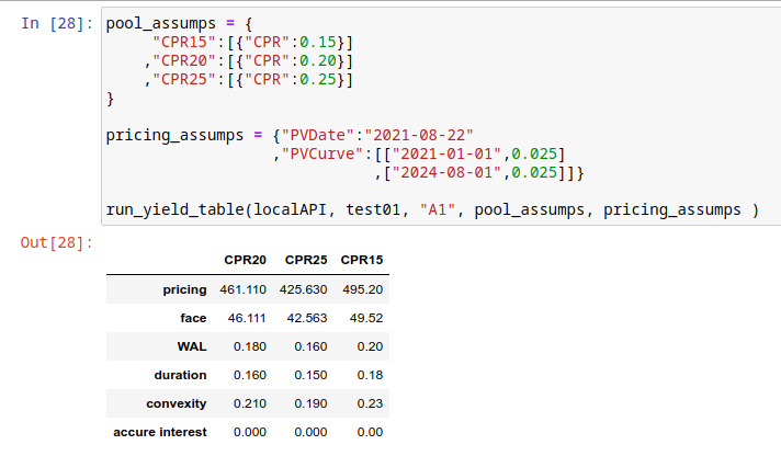
You have it !
How to model cashflow for ARM Mortgage
absbox support ARM mortgage in verison 0.15
with features like:
initPeriod (required) -> using fix rate in first N periods
initial reset cap (optional) -> maxium spread can be jump at first reset date.
periodic reset cap (optional)-> maxium spread can be jump at rest reset dates.
life cap (optional) -> maxium rate during the whole mortgage life cycle
life floor (optional) -> minium rate during the whole mortgage life cycle
from absbox import API

localAPI = API("https://absbox.org/api/latest")

myPool = {'assets':[
            ["AdjustRateMortgage"
            ,{"originBalance": 240.0
             ,"originRate": ["floater"
                             ,0.03
                             ,{"index":"LIBOR1M"
                               ,"spread":0.01
                               ,"reset":["EveryNMonth","2023-11-01",2]}]
             ,"originTerm": 30 ,"freq": "monthly","type": "level"
             ,"originDate": "2023-05-01"
             ,"arm":{"initPeriod":6,"firstCap":0.015} }
            ,{"currentBalance": 240.0
             ,"currentRate": 0.08
             ,"remainTerm": 19
             ,"status": "current"}]],
         'cutoffDate':"2021-03-01"}

localAPI.runPool(myPool,
                 runAssump=[("interest"
                             ,("LIBOR1M",[["2021-01-01",0.05]
                                          ,["2022-02-01",0.055]
                                          ,["2022-07-01",0.0525]
                                          ,["2023-09-01",0.06]
                                          ,["2023-12-15",0.07]
                                          ,["2024-01-15",0.08]
                                          ,["2024-10-15",0.10]]))],
                  read=True)
How to view projected quasi Financial Reports ?
After the deal was run, user can view the cashflow of pool/ bonds fees etc or transaction logs from accounts
#view result of bonds
r['bonds']

#transaction logs of accounts
r['accounts']

#pool cashflow
r['pool']['flow']

#expenses
r['fee']
For the users who is not patient enough or who want to take a high level view of how the deal was changing during the future. absbox support Financial Reports since version 0.17.0.
Syntax
To build the financial reports , user need to add a tuple in the list of runAssump.
("report",{"dates":<DatePattern>})
the <DatePattern> will be used to describe Financial Report Date.
Example:
r = localAPI.run(deal
                ,poolAssump = ("Pool"
                                ,("Mortgage"
                                ,{"CDR":0.01} ,None, None, None)
                                ,None
                                ,None)
                ,runAssump = [("inspect",
                                ("MonthEnd",("cumPoolDefaultedBalance",)))
                              ,("report",
                                {"dates":"MonthEnd"})]
                ,read=True)
Cash Report
Cash Report will list a cash inflows and outflows of the deal. Report was compiled against transaction logs of accounts.
r['result']['report']['cash']
Balancesheet Report
Balancesheet Report will take a snapshot of the deal on the dates described in DatePattern. It will also include the bond interest accured or fee accured as both of them are Payable in the balance sheet .
r['result']['report']['balanceSheet']

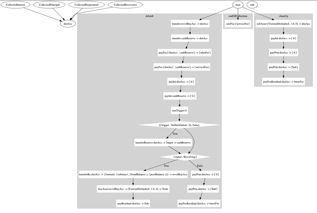
Model a revolving deal (BMW Auto)
Modelling a revolving deal is quite chanllenge , here is an real transaction which highlights the key components
The whole model can be referred to here BMW Auto Deal 2023-01
Revolving Period
The revolving period usually was set like first 12/24 months after closing of deal. While the transaction may impose some other condition to enter Amortization stage when certain criteria was met, like pool cumulative default rate.
In this case, we model such event of entering amortizating with a trigger :
if deal date was later than 2024-05-26 OR
pool cumulative defaulted rate greater than 1.6%,
then change the deal status from Revolving to Amortizing
# a trigger
{"condition":["any"
               ,[">=","2024-05-26"]
               ,[("cumPoolDefaultedRate",),">",0.016]]
 ,"effects":("newStatus","Amortizing")
 ,"status":False
 ,"curable":False}
Once the deal enter a new status Amortizing, then in the waterfall acitons would branch base deal status :
["IfElse"
  ,["status","Revolving"] # the predicate
  ,[["transferBy",{"formula":("substract",("bondBalance",),("poolBalance",))} # list of actions if predicate is True ()
                 ,"distAcc",'revolBuyAcc']
   ,["buyAsset",["Current|Defaulted",1.0,0],"revolBuyAcc",None]
   ,["payIntResidual","distAcc","Sub"] ]
  ,[["payPrin","distAcc",["A"]] # >>>> list of actions if deal is NOT  Revolving Status
   ,["payPrin","distAcc",["Sub"]]
   ,["payFeeResidual", "distAcc", "bmwFee"]]]]
Revolving Asset
Asset to be bought in the future isn’t really part of deal data, thus we are going to supply these dummy asset in the Assumption
Pls noted:
revolving assets to be bought can be a portfolio which means a list of assets .
user can set up a snapshot curve to simulate different assets at points of time in the future to be bought.
user can set different pool performance assumption on the revolving pool
revol_asset = ["Mortgage"
                ,{"originBalance":220,"originRate":["fix",0.043],"originTerm":48
                  ,"freq":"Monthly","type":"Level","originDate":"2021-07-01"}
                  ,{"currentBalance":220
                  ,"currentRate":0.043
                  ,"remainTerm":36
                  ,"status":"current"}]

r = localAPI.run(BMW202301
                ,runAssump = [("revolving"
                                ,["constant",revol_asset]
                                ,("Pool",("Mortgage",{"CDR":0.07},None,None,None)
                                          ,None
                                          ,None))]
                ,read=True)
Revolving Buy
Pricing an revolving asset would have a huge impact on the pool cashflow .
["buyAsset",<PricingMethod>,<Account>,None]
price an asset with balance factor [“Current|Defaulted”,0.95,0] means , if the asset has a current balance of 100, then the price would be 100*0.95 = 95
price an asset with curve, with a pricing curve supplied, price an asset by discount cashflow of the asset
["IfElse"  #
 ,["status","Revolving"]
 ,[["transferBy",{"formula":("substract",("bondBalance",),("poolBalance",))}
                ,"distAcc",'revolBuyAcc']
  ,["buyAsset",["Current|Defaulted",1.0,0],"revolBuyAcc",None] # <--- action of buying revolving assets
  ,["payIntResidual","distAcc","Sub"] ]
 ,[["payPrin","distAcc",["A"]]
  ,["payPrin","distAcc",["Sub"]]
  ,["payFeeResidual", "distAcc", "bmwFee"]]]]
Debug the cashflow
Well.. there isn’t such Debug action on the cashflow, but a more precise put:
a various angles to `View` the cashflow
how to debug cashflow
Stop Run At Certain Date
user can instruct the projection to stop at certian date Stop Run
Error/Warning Log
New in version 0.22.
Hastructure engine will perform certian validation check before or after deal run, user can inspect the log via:
ErrorMeans the run result is in-complete, don’t use the number for downstream
WarningMeans the cashflow projection is complete but subject to unorthodox design
from absbox import API,mkDeal
localAPI = API("http://localhost:8081",check=False)

deal = mkDeal(deal_data,preCheck=False)

r = localAPI.run(deal
                ,poolAssump = None
                ,runAssump = None
                ,read=True
                ,preCheck=False)

r['result']['logs']
Financial Reports
This will offer a high level on how stats chagnes during cashflow projection.
user can inspect Balancesheet and Cashflow report from a highlevel. How to view projected quasi Financial Reports ?
Account transactions
if user want to view the break down of waterfall distribution, user may view account transaction via:
r['accounts']['AccountName01']
Inspect Free Formulas on projection
If user would like to view variables during the cashflow projection, there is a time machine built for this purpose. Inspecting Numbers
User just need to provide :
“When” to view the variables via a DatePattern and
“What” variables to view via a Formula
Inspect Free formulas within waterfall distribution
New in version 0.22.
Note
Free formula in Projection v.s Free formula in Waterfall
- Free formula in Projection
formula value was evaluated at End of Day on dates specified via
DatePattern. The value won’t be changed again in that day.
- Free formula in Waterfall
formula value was evaluated at Point of time on the location in the waterfall. The value may changes if futhur actions were taken in the waterfall in that day.
Joint Inspection Reader
New in version 0.29.13.
User can inspect the variables in BOTH Projection and Waterfall via function readInspect(r['result'])
Which waterfalls has been run?
New in version 0.28.17.
User can inspect the waterfalls has been run via:
r['result']['waterfall']

Visualize the cash flow
Waterfall rules can be complex and headache. Luckily absbox is gentle enough to provide candy function to visualize the fund allocation.
absbox is using Graphviz , pls make sure it was installed as well as python wrapper graphviz
Let’s use the example -> BMW Auto Deal 2023-01
from absbox.local.chart import viz

viz(BMW202301) # that's it ,done !
preview
Project Cashflow for Solar Panel
New in version 0.23.
Fixed Asset
FixedAsset was introduced in absbox version 0.23, which represent a object:
depreciates by Accounting rule
has the ability to produce an amount of something, which can be monetized in the market.
the ability (maxium amount of something produced ) may decay as the asset is depreciating.
But it’s not always producing something in the maxium level, so it will subject to a Utilization Rate curve from input assumption.
And, it can’t sell all the something at same price all over the time, the market price will be read from Price Curve from input assumption.
It looks abstract but indeed provide more coverage to different asset classes, like Solar Panel , Hotel Room etc .
how a fixed Asset generate cash
Solar Panel
Solar Panel is a good example of this type of asset as it fullfill the feactures below:
it produce Electricity as Something, the production of Electricity fluctuates due to seasonality, thus
Utilization RateCurve can be applied.the maxium production capacity is decaying due to the installation equipment depreciates.
The Electricity can be monetized in someway ,and the price may varies, due to supply and demand, thus
Price Curvecan be applied as well.
Build a story
OK, let’s assume ,we are a homeowner that want to install a solar panel system with financing from a loan. Now we are going to build a cashflow deal model to see if it’s a good deal.
Liability & Equity
assuming taking a passthrough loan with rate of 5%
down payment at 40%
Asset & expense
maxium production level : 20kw per day,average sunlight per month 20days.
cost 15000, expect usage life 15 yrs(180 months), residual value at $1000
monthly insurance fee 20
average maintenance cost $200 each year, extra $200 after 10yrs.
assets = [["FixedAsset"
            ,{"start":"2023-11-01","originBalance":15000,"originTerm":240
              ,"residual":1000,"period":"Monthly","amortize":"Straight"
              ,"capacity":("Fixed",20*20*2)}
            ,{"remainTerm":240}]]

exps = (("maintenance",{"type":{"recurFee":["YearFirst",200]}})
        ,("maintenance2",{"type":{"recurFee":["YearFirst",200],"feeStart":"2033-11-01"}})
        ,("insurance",{"type":{"recurFee":["MonthFirst",20]}}))
Waterfall
pay all the expense
pay interest and principal of loan
pay principal to equity tranche but keep fee/insurance at account
when clean up deal , sell the asset and pay prin and yield to equity tranche.
waterfall = {"amortizing":[
                ["payFee","acc01",['maintenance','maintenance2','insurance']]
                ,["accrueAndPayInt","acc01",["A"]]
                ,["payPrin","acc01",["A"]]
                ,["payPrin","acc01",["EQ"]
                  ,{"limit":{"formula":("floorWithZero"
                              ,("substract"
                                ,("accountBalance","acc01"),("constant",1045)))}}]
              ]
            ,"cleanUp":[
                ["sellAsset",["Current|Defaulted",1.0,0],"acc01"]
                ,["payPrin","acc01",["EQ"]]
                ,["payIntResidual","acc01","EQ"]
            ]}
transaction file:
from absbox.local.generic import Generic
from absbox import API
localAPI = API("https://absbox.org/api/dev",lang='english',check=False)

solarPanel = Generic(
  "TEST01"
  ,{"cutoff":"2024-01-01","closing":"2024-01-01","firstPay":"2024-02-01"
   ,"payFreq":"MonthEnd","poolFreq":"MonthEnd","stated":"2050-01-01"}
  ,{'assets':assets}
  ,(("acc01",{"balance":0}),)
  ,(("A",{"balance":9_000
         ,"rate":0.05
         ,"originBalance":9_000
         ,"originRate":0.00
         ,"startDate":"2024-01-01"
         ,"rateType":{"Fixed":0.05}
         ,"bondType":{"Sequential":None}})
    ,("EQ",{"balance":7_000
         ,"rate":0.0
         ,"originBalance":7_000
         ,"originRate":0.00
         ,"startDate":"2024-01-01"
         ,"rateType":{"Fixed":0.00}
         ,"bondType":{"Equity":None}}),
   )
  ,exps
  ,waterfall
  ,[["CollectedCash","acc01"]]
  ,None
  ,None
  ,None
  ,None
  ,("PreClosing","Amortizing")
  )
Project Cashflow
Nowe we need assumption to project cashflow:
Assumption
utility rate, utility rate start first year at 90% and 85% second year, then stable at 80%
price of Electricity, fixed price first year at 0.3 and drop down 0.5 each year and remains at 0.2
call the deal at
2044,20yrs later
myAssump = ("Pool"
            ,("Fixed",[["2024-01-01",0.3]
                      ,["2025-01-01",0.25]
                      ,["2026-01-01",0.2]]
                     ,[["2024-01-01",0.9]
                      ,["2025-01-01",0.85]
                      ,["2026-01-01",0.8]])
            ,None
            ,None)

p = localAPI.run(solarPanel,poolAssump=myAssump
                      ,runAssump=[("call",{"afterDate":"2044-01-01"})
                                  ,("report",{"dates":"MonthEnd"})]
                      ,read=True)
we can inspect the cashflow projection :ref: and calculate the IRR of equity investment:
from absbox.local.analytics import irr
irr(p['bonds']['EQ'],init=('2024-01-01',-7_000))
it was 1.67% (YoY)…whoa…sad
Sensitivity Analysis
Well, things won’t work out as planned, what happen if price fall down ? or the utilization rate fall ?
We can perform sensitivity analysis to explore how robust our investment is
scenarioMap = {
  "base":("Pool"
          ,("Fixed",[["2024-01-01",0.3]
                    ,["2025-01-01",0.25]
                    ,["2026-01-01",0.2]]
                   ,[["2024-01-01",0.9]
                    ,["2025-01-01",0.85]
                    ,["2026-01-01",0.8]])
          ,None
          ,None)
  ,"lowUtil" :("Pool"
              ,("Fixed",[["2024-01-01",0.3]
                        ,["2025-01-01",0.25]
                        ,["2026-01-01",0.2]]
                       ,[["2024-01-01",0.85]
                        ,["2025-01-01",0.80]
                        ,["2026-01-01",0.75]])
              ,None
              ,None)
 ,"lowPrice" : ("Pool"
              ,("Fixed",[["2024-01-01",0.3]
                        ,["2025-01-01",0.225]
                        ,["2026-01-01",0.19]]
                       ,[["2024-01-01",0.9]
                        ,["2025-01-01",0.85]
                        ,["2026-01-01",0.8]])
              ,None
              ,None)
 }
 p = localAPI.run(solarPanel,poolAssump=scenarioMap
                     ,runAssump=[("call",{"afterDate":"2044-01-01"})
                                ,("report",{"dates":"MonthEnd"})]
                     ,read=True)
from absbox.local.util import irr
{k:irr(v['bonds']['EQ'],init=('2024-01-01',-7000))
  for k,v in p.items()}

#  {'base': 0.016930937065270275,
#   'lowPrice': 0.0028372850153230164,
#   'lowUtil': -0.0013152392627518972}
Well, it’s pretty clear that in current transaction , lower price isn’t most scary factor comparing to low utilization rate. In the long run of 20 years, keep higher utilization rate is important, so sweep the panel weekly!
or you can buy a robot to do that ,but it will drag down the IRR :)
Conclusion
Making an installation of roof solar panel is a big investment decision which involves pretty long time horizon and calculation of factor like electricity price as well as loan rate.
It may look easier if you can build a cashflow model and perform quantitative analysis to support the decision !
Happy hacking !
Other Asset types
The FixedAsset type can be used to model assets as well. For example ,
Hotel
We can model a hotel as FixedAsset ,whose capacity is the all rooms available for booking. When projects cashflow , we provide assumptions
utility rate curve -> on average ,how many rooms served during the Period.
price curve -> average price per night during the Period, which may reflect seasonality flucturation.
The multiplication of two would be the cashflow generated from this asset.
EV charger station
same with Hotel
How to use Deal Library
What is Deal Library?
Deal Library is a collection of deal objects, which can be used to store and retrieve deal objects.
As deal objects is actually represented in JSON , it can be easily stored in a Non-SQL database like MongoDB or CouchDB or even AWS S3 or Azure Blob Storage.
Given a customizied tagging , user can easily retrieve the deal objects with criteria from the library.
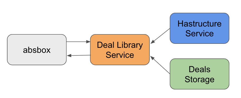
Note
The Deal Library Service / Deals Storage / Hastructure can be deployed in a self-host environment.
How to build a deal library?
absbox.org provide a deal library service, user can store and retrieve deal objects via absbox API.
Users have the option to build their own Deal Library or just deploy the service(code is available but offering is subjected to a commercial agreement) in self-host environment to minimise the security risk.
How to use a deal library?
User just need to pass the bond id and pool/deal level assumptions to the runLibrary() function, the deal object will be retrieved from the library and projected cashflow will be returned.
Why using a deal library ?
seperating deal storages and deal calculation engine, which is good for security and performance.
seperating running assumption and deal calculation, which is good for reusability and maintainability.
How to pass deal files around ?
A deal object
A deal object either initialized with SPV or Generic class, is actually a python dataclass which implements a .json() .
The json() function will convert the class to a json representation string .
A string
Now with that string, user can just write it into a No-SQL document database . or sent via Email , or Fax it .
How to use Deal JSON string
The JSON string from .json() method can be used as part of post request send to Hastructure engine.
But unfortunately there is no way convert the string back to python class so far.
Primary Pricing with Absbox
Primary Pricing is a process of calculating the price of a bond at the time of issuance.
Tempalte: Model CLO
Warning
Working in progess
CLO features:
Quarterly Payment
Floating Rate of assets and liabilities
IC/OC/IDT test
Interest & Principal Waterfall
How to get response ?
Typically, a function call has parameter read
read = True
If user supplied with True, absbox will try to convert response with pandas dataframe where possible.
read = False
Or, use can pass with read with False, which will just return a raw response from servant/aeson.
To make it slightly readable , there is a util function may help.
New in version 0.42.6.
from absbox import readAeson

r0 = localAPI.run(.....,read=False)

readAeson(r0)
How to use pre-built executable
Download executable
Go to the Release link and download the executable for your OS.
Download the config.yaml as well
Put both files in the same folder.
Mac OS
Windows
Linux/Ubuntu/Debian
Verify
The console shall show running message

open a browser or cURL to make a get request to
http://localhost:8081/version
Note
The port number can be changed in config.yaml
curl http://localhost:8081/version
